Tutorials

This is a list of step-by-step tutorials that will help you get started. The tutorials are based on state of the art methods with publicly available code.

FlowDenoising Deployment

This tutorial shows how to prepare and deploy an algorithm to Compox and run it in Tescan 3D Viewer (and optionally Tescan Picannto). We’ll use the FlowDenoising algorithm from GitHub as an example. The FlowDenoising algorithm suppresses high-frequency noise using an optical-flow-driven Gaussian kernel. The FlowDenoising source code is distributed under the terms of the GNU General Public License v3.0 (GPL-3.0).

V. González-Ruiz, M.R. Fernández-Fernández, J.J. Fernández.
Structure-preserving Gaussian denoising of FIB-SEM volumes.
Ultramicroscopy 246, 113674 (2023).
DOI: 10.1016/j.ultramic.2022.113674

Visualization

1. Compox Installation

For managing dependencies, we recommend using uv — it’s fast and automatically handles both your environment and package versions. You can install it by this command:

pip install uv

You can set up your project and environment by running this command in your project’s root directory:

uv init

Next, activate the project virtual environment:

.\.venv\Scripts\Activate.ps1

Once the environment is ready, install Compox using:

uv add compox

Generate a server config:

compox generate-config --path app_server.yaml

Config app_server.yaml should appear in project’s root directory. Now create an empty folder called algorithms in your project’s root directory. You now have everything ready to start creating algorithms.

project_root/
├── algorithms/
└── app_server.yaml

2. Importing FlowDenoising as submodule

Create an algorithm root directory inside algorithms directory. We’ll call it flow_denoising:

From within this new directory, you can download the algorithm’s source code from GitHub into a subfolder named files by running:

git submodule add https://github.com/ElsevierSoftwareX/SOFTX-D-23-00180.git files

After importing the submodule, your project structure should look like this:

project_root/
├── algorithms/
│   └── flow_denoising/
│       └── files/
│           ├── manual/...
│           ├── src/...
│           └── LICENCE.txt
└── app_server.yaml

The repository includes a requirements.txt at algorithms/flow_denoising/files/src/requirements.txt. Install the dependencies:

uv add --requirements algorithms/flow_denoising/files/src/requirements.txt

3. Creating the `pyproject.toml` file

The pyproject.toml file contains metadata and configuration for your algorithm. It is used by Compox during the deployment process to register the algorithm as a service. Place it in the flow_denoising directory:

project_root/
├── algorithms/
│   └── flow_denoising/
│       ├── files/
│       │   ├── manual/...
│       │   ├── src/...
│       │   └── LICENCE.txt
│       └── pyproject.toml
└── app_server.yaml

[project] section – basic package information

This section defines general information about your algorithm. At minimum, you must include the name and version fields. The version follows the major.minor.patch format (e.g. 0.1.0).

[project]
name = "flow_denoising"
version = "0.1.0"

[tool.compox] section – Algorithm-specific configuration

This section contains settings used by Compox itself — how your algorithm behaves, what devices it supports, and which parameters users can configure. Although all fields here are optional, it’s recommended to include them for better integration and usability.

[tool.compox]
algorithm_type = "Image2Image"
tags = ["image-denoising", "Image2Image"]
description = "Removes most of the high-frequency components of the data using a Optical-Flow-driven Gaussian kernel with abilities to preserve the structures and avoid blurring, and outputs the filtered volume"
supported_devices = ["cpu", "gpu"]
default_device = "cpu"
additional_parameters = [
    {name = "sigmas", description = "Standard deviations of the Gaussian kernel in each dimension.", config = {type = "int_list", default = [1, 1, 1], adjustable = true}},
    {name = "level", description = "Level parameter for optical flow filtering.", config = {type = "int", default = 3, adjustable = true}},
    {name = "winsize", description = "Window size parameter for optical flow filtering.", config = {type = "int", default = 7, adjustable = true}},
    {name = "optical_flow", description = "Enable or disable optical flow filtering.", config = {type = "bool", default = true, adjustable = true}},]

check_importable = false
obfuscate = true
hash_module = true
hash_assets = true

Explanation of key fields:

For a detailed explanation of all [tool.compox] fields, see the How to create an algorithm module.

4. Creating `Runner.py`

Runner.py is the entry point Compox calls to execute your algorithm. Place it in algorithms/flow_denoising:

project_root/
├── algorithms/
│   └── flow_denoising/
│       ├── files/
│       │   ├── manual/...
│       │   ├── src/...
│       │   └── LICENCE.txt
│       ├── pyproject.toml
│       └──Runner.py
└── app_server.yaml

Importing dependencies

For this example, we’ll use NumPy for numerical operations. Make sure it is installed in your environment (if not, you can add it with):

uv add numpy

Since this algorithm is of type Image2Image, we will inherit from Image2ImageRunner, which can be imported from compox.algorithm_utils.Image2ImageRunner.

For debugging, we can also import the helper function debug from compox.algorithm_debug.

From the FlowDenoising source code (in the submodule files/src/flowdenoising_sequential), we will use three main functions:

get_gaussian_kernel
OF_filter
no_OF_filter

Here’s the complete set of imports:

import numpy as np

from files.src.flowdenoising_sequential import get_gaussian_kernel, OF_filter, no_OF_filter
from compox.algorithm_utils.Image2ImageRunner import Image2ImageRunner
from compox.algorithm_debug import debug

Initializing the `Runner` class

As mentioned earlier, the Runner class should inherit from Image2ImageRunner. This base class already handles data fetching, preprocessing, and uploading the results back. For this algorithm, you only need to override the inference method. It receives the input data as an np.ndarray together with a dict of parameters, and must return the processed data as an np.ndarray. If you want to customize how data is fetched or uploaded, you can override these methods yourself or inherit directly from BaseRunner. For more details, see How to create an algorithm module.

A minimal skeleton looks like this:

class Runner(Image2ImageRunner):

    def inference(self, input_data: np.ndarray, args: dict | None = None) -> np.ndarray:
        pass

Implementing FlowDenoising in the `inference` method

First, extract all user-defined parameters from the input dictionary args:

# Extract parameters
sigmas = args["sigmas"]
l = args["level"] 
w =  args["winsize"]
optical_flow = args["optical_flow"]

Next, compute Gaussian kernels for each dimension:

# Create Gaussian kernels for each dimension
k_x = get_gaussian_kernel(int(sigmas[0]))
k_y = get_gaussian_kernel(int(sigmas[1]))
k_z = get_gaussian_kernel(int(sigmas[2]))
kernel = [k_x, k_y, k_z]

Depending on the boolean value of optical_flow, apply the appropriate FlowDenoising function to the input data:

# Apply filtering
if optical_flow == True:
    filtered_vol = OF_filter(input_data, kernel, l, w)
else:
    filtered_vol = no_OF_filter(input_data, kernel)

Finally, ensure the output is of type float32 and normalized to the range [0, 1]:

# Ensure output data is float32
out_data = filtered_vol.astype(np.float32).copy()

# Normalize output data to [0, 1]
vmin = float(np.nanmin(out_data))
vmax = float(np.nanmax(out_data))
if vmax > vmin:
    out_data = (out_data - vmin) / (vmax - vmin)
else:
    out_data[:] = 0.0

return out_data

Full example: Runner.py

import numpy as np

from files.src.flowdenoising_sequential import get_gaussian_kernel, OF_filter, no_OF_filter
from compox.algorithm_utils.Image2ImageRunner import Image2ImageRunner
from compox.algorithm_debug import debug

class Runner(Image2ImageRunner):

    def inference(self, input_data: np.ndarray, args: dict | None = None) -> np.ndarray:

        # Extract parameters
        sigmas = args["sigmas"]
        l = args["level"] 
        w =  args["winsize"]
        optical_flow = args["optical_flow"]

        # Create Gaussian kernels for each dimension
        k_x = get_gaussian_kernel(int(sigmas[0]))
        k_y = get_gaussian_kernel(int(sigmas[1]))
        k_z = get_gaussian_kernel(int(sigmas[2]))
        kernel = [k_x, k_y, k_z]

        # Apply filtering
        if optical_flow == True:
            filtered_vol = OF_filter(input_data, kernel, l, w)
        else:
            filtered_vol = no_OF_filter(input_data, kernel)

        # Ensure output data is float32
        out_data = filtered_vol.astype(np.float32).copy()

        # Normalize output data to [0, 1]
        vmin = float(np.nanmin(out_data))
        vmax = float(np.nanmax(out_data))
        if vmax > vmin:
            out_data = (out_data - vmin) / (vmax - vmin)
        else:
            out_data[:] = 0.0

        return out_data

5. Debugging `Runner.py`

Once your first implementation is ready, you will likely want to run it on a small data sample with debugging support to verify its behavior. The compox.algorithm_debug.debug function allows you to test your algorithm without launching Tescan 3D Viewer. It does not load data the same way as the Viewer — the debug tool simply reads the input files directly from disk. However, the rest of the execution pipeline behaves the same: the data is stored in the database, then the preprocess, inference, and postprocess steps run in the same order, and the results are uploaded back to the database. If everything completes successfully, you should see an output similar to this:

2025-11-27 15:04:58.393 | INFO     | compox.algorithm_utils.BaseRunner:run:244 - Starting execution.
2025-11-27 15:04:58.395 | INFO     | compox.algorithm_utils.BaseRunner:preprocess_base:287 - Data preprocessing finished in 0.0 seconds
2025-11-27 15:04:58.395 | INFO     | compox.algorithm_utils.BaseRunner:inference_base:336 - Running inference.
2025-11-27 15:05:00.192 | INFO     | compox.algorithm_utils.BaseRunner:inference_base:339 - Inference finished in 1.8 seconds
2025-11-27 15:05:00.192 | INFO     | compox.algorithm_utils.BaseRunner:postprocess_base:386 - Postprocessing output data.
2025-11-27 15:05:00.192 | INFO     | compox.tasks.TaskHandler:post_data:904 - Uploading 6 results to the database.
2025-11-27 15:05:00.192 | INFO     | compox.algorithm_utils.BaseRunner:postprocess_base:389 - Postprocessing finished in 0.0 seconds
2025-11-27 15:05:00.192 | INFO     | compox.algorithm_utils.BaseRunner:run:253 - Execution completed in 1.8 seconds.
2025-11-27 15:05:00.192 | INFO     | compox.tasks.TaskHandler:_log_file_stats:402 - File fetching stats: 6.0 files fetched in 0.0010 seconds.
2025-11-27 15:05:00.192 | INFO     | compox.tasks.TaskHandler:_log_file_stats:406 - File posting stats: 6.0 files posted in 0.0000 seconds.

Debug function inputs

The debug function accepts four inputs:

data – path to a dataset on your local disk. This can be either path to folder containing image slices (.jpg, .png, .tiff), or a 3D volume (.tiff, .npy, .hdf5).
algo – path to the root directory of your algorithm.
params – a dictionary containing additional algorithm parameters.
device – compute device to run the algorithm on (e.g., "cpu" or "gpu").

You can use your own data, or you can use one of the sample datasets included in Tescan 3D Viewer.
For example, the Oscillatoria dataset can be downloaded from the Welcome Page of the Viewer.

Sample Dataset

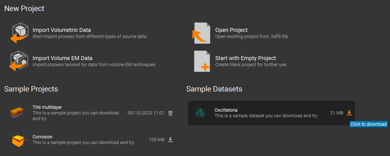
Its default location is:

`...\User\Documents\TESCAN GROUP, a.s.\Tescan 3D Viewer\Sample projects and datasets\Oscillatoria_dataset\Oscillatoria3D.tif`. 

You can also import any dataset into the Viewer, crop it, export it, and then use that exported data for debugging.

Running debug tool

You have two main options for debugging:

Running your script in debug mode with compox.algorithm_debug.debug()
Debug through the CLI

Option 1: Use the `debug()` Function

Add this code block at the bottom of your Runner.py and run it in your IDE (e.g. VS Code, PyCharm). When running Runner.py directly.

if __name__ == "__main__":
    debug(
        algo_dir="algorithms/flow_denoising",
        data="path to data",
        params={"sigmas": [1, 1, 1], "level": 3, "winsize": 7, "optical_flow": True},
        device="cpu",
    )

You can also use Python’s built-in debugger — simply insert a breakpoint() wherever you want to pause execution and run script manually:

uv run .\algorithms\flow_denoising\Runner.py

Option 2: Debug through the CLI

Just insert breakpoint() wherever you want to pause execution. Then run your algorithm from the terminal like this:

compox debug run --data "path to data" --algo "path to Flowdenoising algorithm" --device "cpu" --param sigmas=[1,1,1] --param level=3 --param winsize=7  --param optical_flow=true

Visualization of filtered data

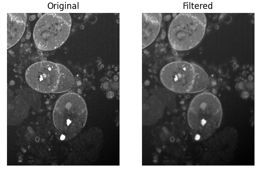
If you want to visually compare the original and filtered data during debugging, you can add a small helper method to your Runner class. For example:

import matplotlib.pyplot as plt

def visualize(self, input_data, filtered_vol):
        plt.subplot(1, 2, 1)
        plt.imshow(input_data[input_data.shape[0] // 2, :, :], cmap='gray')
        plt.title("Original")
        plt.axis('off')

        plt.subplot(1, 2, 2)
        plt.imshow(filtered_vol[filtered_vol.shape[0] // 2, :, :], cmap='gray')
        plt.title("Filtered")
        plt.axis('off')

        plt.show()

To show this result only when debugging, we recommend using an environment variable. You can set it in the __main__ block:

import os

if __name__ == "__main__":
    os.environ["COMPOX_DEBUG_SHOW"] = "1"
    debug(
        algo_dir="algorithms/flow_denoising",
        data="path to data",
        params={"sigmas": [1, 1, 1], "level": 3, "winsize": 7, "optical_flow": True},
        device="cpu",
    )

Then, in your inference method, call the visualize function only when this environment variable is set:

if os.getenv("COMPOX_DEBUG_SHOW") == "1":
    self.visualize(input_data, filtered_vol)

This way, the visualization will appear when you run Runner.py directly for debugging, but it will not show any extra windows when the algorithm is executed from Tescan 3D Viewer. After running, you should see a side-by-side comparison of the original and filtered slices:

Visualization

6. Updating the progress bar in Viewer during inference

This step is optional. By default, the Viewer already displays a progress bar that is updated during most stages of the algorithm execution. However, during the inference step the progress bar is not updated and only continues once inference is fully completed.

Simple progress updates inside `inference`

You can update the progress bar from anywhere inside the inference method using the set_progress function. The function accepts a floating-point value in the range 0.0 – 1.0, representing the overall progress.

# Extract parameters
sigmas = args["sigmas"]
l = args["level"] 
w =  args["winsize"]
optical_flow = args["optical_flow"]
self.set_progress(0.2)

# Create Gaussian kernels for each dimension
k_x = get_gaussian_kernel(int(sigmas[0]))
k_y = get_gaussian_kernel(int(sigmas[1]))
k_z = get_gaussian_kernel(int(sigmas[2]))
kernel = [k_x, k_y, k_z]
self.set_progress(0.3)

# Apply filtering
if optical_flow == True:
    filtered_vol = OF_filter(input_data, kernel, l, w)
else:
    filtered_vol = no_OF_filter(input_data, kernel)
self.set_progress(0.9)

The estimated remaining time is computed automatically by the Viewer based on how often and how smoothly the progress value is updated.

More accurate progress updates using callbacks

In the FlowDenoising algorithm, most of the execution time is spent inside the OF_filter function. To obtain a more accurate progress estimation, the progress bar can be updated during the filtering itself, based on how much data has already been processed. This can be achieved by introducing a progress callback that is called repeatedly during processing.

Creating a progress callback helper

Add the following helper method to the Runner class:

def make_progress_callback(self, start, end):
        span = end - start

        def callback(frac):
            frac_clamped = max(0.0, min(1.0, float(frac)))
            self.set_progress(start + span * frac_clamped)

        return callback

This helper creates a callback function that maps a fractional progress value (0.0 – 1.0) into a selected range of the global progress bar.

Passing the callback into `OF_filter`

Next, create a progress callback instance and pass it into OF_filter. For simplicity, we map the entire inference step to the full progress range 0.0 – 1.0:

# Apply filtering
progress_callback = self.make_progress_callback(0.0, 1.0)
if optical_flow == True:
    filtered_vol = OF_filter(input_data, kernel, l, w, progress_callback)
else:
    filtered_vol = no_OF_filter(input_data, kernel)

Propagating progress through the filtering implementation

To enable progress reporting inside the filtering code, the original implementation of OF_filter must be extended to accept the callback and propagate it to all axis-specific filtering functions.

def OF_filter(vol, kernel, l, w, progress_callback):
    mean = vol.mean()
    filtered_vol_Z = OF_filter_along_Z(vol, kernel[0], l, w, mean, axis_progress_callback=progress_callback)
    filtered_vol_ZY = OF_filter_along_Y(filtered_vol_Z, kernel[1], l, w, mean, axis_progress_callback=progress_callback)
    filtered_vol_ZYX = OF_filter_along_X(filtered_vol_ZY, kernel[2], l, w, mean, axis_progress_callback=progress_callback)

    return filtered_vol_ZYX

Reporting progress per axis

For progress reporting inside each axis loop, add the following helper function near the top of flowdenoising_sequential.py:

def report_axis_progress(axis_progress_callback, axis, slice_idx, number_of_slices, axes = 3):
    if axis_progress_callback is None or number_of_slices <= 0:
        return
    base = axis / axes
    span = 1.0 / axes
    frac = (slice_idx + 1) / number_of_slices
    axis_progress_callback(base + span * frac)

For simplicity, this implementation assumes that processing time is evenly distributed across all axes.

Calling progress reporting inside axis filters

Finally, call report_axis_progress from inside each axis-specific filtering function. Example for filtering along the Z axis:

def OF_filter_along_Z(vol, kernel, l, w, mean, axis_progress_callback=None):
    ...
    for z in range(Z_dim):
        ...
        report_axis_progress(axis_progress_callback, 0, z, Z_dim)

    return filtered_vol

For the remaining axes:

report_axis_progress(axis_progress_callback, 1, y, Y_dim)

report_axis_progress(axis_progress_callback, 2, x, X_dim)

This approach provides smooth and meaningful progress updates during inference, even for large volumetric datasets. A similar approach can also be applied to the no_OF_filter function if needed.

7. Algorithm Deployment

Once your algorithm is implemented and ready, you can deploy it to Compox using two options:

Single command
GUI

Option 1: Deploy with single command

Simply run this command:

compox deploy-algorithms --config app_server.yaml --name flow_denoising

If you are running the server for the first time, the process might take a bit longer because Compox needs to download and initialize the MinIO service.

Option 2: Deploy with GUI

As an alternative, you can use the built-in Compox GUI to manage algorithms more conveniently. First, edit your app_server.yaml file and enable GUI controls by setting the following values in the gui section:

gui:
  algorithm_add_remove_in_menus: true
  use_systray: true

Then start the Compox server with:

compox run --config app_server.yaml

After running this command, you should see the Compox icon appear in the system tray:

SysTray

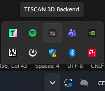
Right-click the icon to open the context menu. From there, you can:

View all currently deployed algorithms
Add a new algorithm by selecting its folder (in our case, choose algorithms/flow_denoising)

Stopping the Server

If you are using the GUI, right-click the tray icon and select Quit to stop the server. Using Ctrl + C in the terminal will not close the server properly when the GUI mode is active.
If you are running from the terminal (without GUI), you can simply press Ctrl + C.

8. Running FlowDenoising in `TESCAN 3D Viewer`

After deploying the algorithm to Compox, you can run it directly on data loaded in TESCAN 3D Viewer.

Step 1: Start the Compox server

Before launching Tescan 3D Viewer, make sure the Compox is running. Start the server with:

compox run --config app_server.yaml

Step 2: Connect `Tescan 3D Viewer` to Compox

After starting the server, open Tescan 3D Viewer. If you see an error saying that the Compox backend connection failed, don’t worry — you can fix this by adding a new backend manually:

Go to Menu → Tools → Preferences
Click Add new backend
Set the Protocol type to HTTP
Check the Custom checkbox
Set the Port number based on your app_server.yaml file
- The default port is 5481
- If you changed it, you can verify the value in the first line of app_server.yaml

Your Preferences window should now look like this:

Preferences

Step 3: Run the algorithm from the Compox extension

Once the backend is connected, import your dataset in Tescan 3D Viewer.

Then open the Compox Backend Extension by clicking the Compox icon in the upper-right corner of the interface.

Preferences

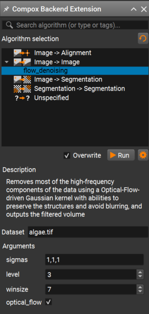
In the Compox Backend Extension window you can:

Select the algorithm you want to run
Read its description
Adjust parameters defined in your pyproject.toml file

After setting the parameters, click Run to start the inference. A progress bar should appear, and the algorithm will run on your dataset.

ParticleSeg3D Deployment

This tutorial describes how to prepare and deploy an algorithm into Compox and run it in TESCAN Picannto. As an example, we use ParticleSeg3D algorithm from GitHub. The ParticleSeg3D is an instance segmentation method that extracts individual particles from large micro CT images based on nnU-Net framework. The source code is distributed under the terms of the Apache Software License 2.0.

Gotkowski, K., Gupta, S., Godinho, J. R. A., Tochtrop, C. G. S.,
Maier-Hein, K. H., & Isensee, F. (2024).
ParticleSeg3D: A scalable out-of-the-box deep learning segmentation solution for individual particle characterization from micro CT images in mineral processing and recycling.
Powder Technology, 434, 119286.
https://doi.org/10.1016/j.powtec.2023.119286

Visualization

1. Compox Installation

For managing dependencies, we recommend using uv — it’s fast and automatically handles both your environment and package versions. You can install it by this command:

pip install uv

You can set up your project and environment by running this command in your project’s root directory:

uv init

ParticleSeg3D is known to work reliably with Python 3.10. With newer Python versions you may run into dependency/build issues, so we recommend creating a dedicated Python 3.10 virtual environment:

uv venv .venv --python=3.10

Next, activate the project virtual environment:

.\.venv\Scripts\Activate.ps1

Once the environment is ready, install Compox using:

uv add compox

Generate a server config:

compox generate-config --path app_server.yaml

Config app_server.yaml should appear in project’s root directory. Now create an empty folder called algorithms in your project’s root directory. You now have everything ready to start creating algorithms.

project_root/
├── algorithms/
└── app_server.yaml

2. Importing ParticleSeg3D as submodule

From the project root directory, download the algorithm source code from GitHub into a subfolder named external:

git submodule add https://github.com/MIC-DKFZ/ParticleSeg3D.git external 

ParticleSeg3D requires pretrained model weights for inference. Download the model weights from here. After downloading, extract the archive and place the directory Task310_particle_seg into algorithms/particle_seg_3d/assets.

Some dependencies used by ParticleSeg3D rely on the pkg_resources module which was removed in recent versions. To avoid this issue, explicitly pin setuptools to a compatible version before installing other dependencies:

uv add "setuptools==80.8.0"

Then install the ParticleSeg3D dependencies from the external directory in editable mode:

cd external
python -m pip install -e .

If the installation fails with GeodisTK build error, retry the installation with build isolation disabled:

python -m pip install -e . --no-build-isolation

After importing the submodule and downloading model weights your project structure should look like this:

project_root/
├── algorithms/
│   └── particle_seg_3d/
│       └── assets
│           └── Task310_particle_seg/
│               └── nnUNetTrainerV2_slimDA5_touchV5__nnUNetPlansv2.1/...
├── external/...
└── app_server.yaml

3. Creating the `pyproject.toml` file

The pyproject.toml file contains metadata and configuration for your algorithm. It is used by Compox during the deployment process to register the algorithm as a service. Place it in the particle_seg_3d directory:

project_root/
├── algorithms/
│   └── particle_seg_3d/
│       ├── assets
│       │   └── Task310_particle_seg/
│       │       └── nnUNetTrainerV2_slimDA5_touchV5__nnUNetPlansv2.1/...
│       └── pyproject.toml
├── external/...
└── app_server.yaml

[project] section – basic package information

This section defines general information about your algorithm. At minimum, you must include the name and version fields. The version follows the major.minor.patch format (e.g. 0.1.0).

[project]
name = "particle_seg_3d"
version = "0.1.0"

[tool.compox] section – Algorithm-specific configuration

This section contains settings used by Compox itself — how your algorithm behaves, what devices it supports, and which parameters users can configure. Although all fields here are optional, it’s recommended to include them for better integration and usability.

[tool.compox]
algorithm_type = "Image2Segmentation"
tags = ["instance-segmentation", "Image2Segmentation", "segmentation"]
description = "ParticleSeg3D is an instance segmentation method that extracts individual particles from large images."
supported_devices = ["cpu", "gpu"]
default_device = "gpu"
additional_parameters = [
{name = "particle_size", description = "Size of the particles to segment.", config = {type = "float", default = 1.00, adjustable = true}},
{name = "spacing", description = "Image spacing", config = {type = "float", default = 0.01, adjustable = true}}
]

check_importable = false
obfuscate = true
hash_module = true
hash_assets = true

Explanation of key fields:

For a detailed explanation of all [tool.compox] fields, see the How to create an algorithm module.

4. Creating `Runner.py`

Runner.py is the entry point Compox calls to execute your algorithm. Place it in algorithms/particle_seg_3d:

project_root/
├── algorithms/
│   └── particle_seg_3d/
│       ├── assets
│       │   └── Task310_particle_seg/
│       │       └── nnUNetTrainerV2_slimDA5_touchV5__nnUNetPlansv2.1/...
│       ├── pyproject.toml
│       └── Runner.py
├── external/...
└── app_server.yaml

Importing dependencies

This example uses NumPy, Zarr, pathlib, tempfile, json, pickle, os, matplotlib and shutil. If you are missing any dependencies, install them with:

uv add numpy zarr matplotlib

Since this algorithm is of type Image2Segmentation, we will inherit from Image2SegmentationRunner, which can be imported from compox.algorithm_utils.Image2SegmentationRunner.

From the installed ParticleSeg3D source code (in the submodule project_root/external/) we will use function predict_cases and class Nnunet:

Here’s the complete set of imports:

import numpy as np
import zarr
import pytorch_lightning as pl
from pathlib import Path
import tempfile
import json
import shutil
import pickle
import os
import io
import torch
import torch.nn as nn

from compox.algorithm_utils.Image2SegmentationRunner import Image2SegmentationRunner
from particleseg3d.inference.inference import predict_cases
from particleseg3d.inference.model_nnunet import Nnunet

Additional dependencies are PyTorch and CUDA for running the algorithm on a GPU. PyTorch can be installed using the official instructions available here. However, newer versions of PyTorch or CUDA may not be fully compatible with ParticleSeg3D. For this reason, we recommend installing the following tested versions, which are known to work correctly with this algorithm:

uv pip install --index-url https://download.pytorch.org/whl/cu121 "torch==2.5.1" "torchvision==0.20.1"

Initializing the `Runner` class

As mentioned earlier, the Runner class should inherit from Image2SegmentationRunner. This base class already handles data fetching, preprocessing, and uploading the results back. For this algorithm, you only need to override the inference and load_assets methods. inference method receives the input data as an np.ndarray together with a dict of parameters, and must return the processed data as an np.ndarray. load_assets is called once when the Runner instance is created. Assets loaded there are cached together with the Runner, so model weights don’t have to be reloaded on every inference call. If you want to customize how data is fetched or uploaded, you can override these methods yourself or inherit directly from BaseRunner. For more details, see How to create an algorithm module.

A minimal skeleton looks like this:

class Runner(Image2SegmentationRunner):
    
    def inference(self, input_data: np.ndarray, args: dict | None = None) -> np.ndarray:
        pass

Implementing ParticleSeg3D in the `inference` method

First, we need to create a helper function for preparing the data. The model expects the input data to be stored as Zarr. This method can be added to the Runner class:

def prepare_data(self, input_data: np.ndarray, args: dict) -> tuple[Path, Path]:

    # Temp directory for Zarr store
    tmpdir = tempfile.mkdtemp()
    zarr_path = Path(tmpdir)

    # Save input data as Zarr
    images_path = (zarr_path / "images/data.zarr")
    images_path.parent.mkdir(parents=True, exist_ok=True)
    zarr.save(images_path, input_data.astype("float64"))

    # Create JSON metadata
    metadata = {
        "data": {
            "spacing": args["spacing"],
            "particle_size": args["particle_size"],
        }
    }
    metadata_path = zarr_path / "metadata.json"
    with open(metadata_path, "w") as f:
        json.dump(metadata, f, indent=4)

    # Prepare output path
    output_path = (zarr_path / "output")
    output_path.mkdir(parents=True, exist_ok=True)

    return zarr_path, output_path

This helper function creates a temporary directory, stores the input np.ndarray as a Zarr dataset, writes the required JSON metadata using user-provided parameters (spacing, particle_size), and prepares an output directory for the model prediction results.

Next, override load_assets function to save model weights to storage as assets. Prepare config, trainer and setup model for inference.

def load_assets(self) -> None:
    model_dir = "assets/Task310_particle_seg/nnUNetTrainerV2_slimDA5_touchV5__nnUNetPlansv2.1/"
    # Load model config
    pkl_path = os.path.join(model_dir, "plans.pkl")
    asset_pkl = self.fetch_asset(pkl_path)
    self.config = pickle.load(asset_pkl)

    # prepare Trainer
    self.trainer = pl.Trainer(gpus=1, precision=16, logger=False)

    # prepare Mode
    folds_assets = []
    json_assets = []
    for fold in range(5):
        # Load model for each fold
        fold_path = os.path.join(model_dir, f"fold_{fold}/model_best.model")
        fold_asset = self.fetch_asset(fold_path)
        folds_assets.append(fold_asset)
        
        # Load json config for each fold
        json_path = os.path.join(model_dir, f"fold_{fold}/debug.json")
        json_asset = self.fetch_asset(json_path)
        json_assets.append(json_asset)
    self.model = ParticleSegNnUNet(folds_assets, json_assets)
    self.model.eval()

The original Nnunet implementation expects a filesystem path and reads debug.json and model_best.model directly from disk. Because we load these files as assets, we create a small subclass that initializes the network ensemble from asset data instead of a directory path. To do this, create a new class ParticleSegNnUNet that inherits from Nnunet and place it in Runner.py.

class ParticleSegNnUNet(Nnunet):
    def __init__(self, folds_assets, json_assets, device: str = "cuda") -> None:
        pl.LightningModule.__init__(self)

        self.nnunet_trainer = "nnUNetTrainerV2__nnUNetPlansv2.1"
        self.network = self._load_from_assets(folds_assets, json_assets)
        self.final_activation = nn.Softmax(dim=2)
        self.tta = True

    def _load_from_assets(self, folds_assets, json_assets) -> nn.ModuleList:
        ensemble = []
        for ckpt_obj, json_obj in zip(folds_assets, json_assets):
            # Load model config from json
            json_stream = io.TextIOWrapper(json_obj, encoding="utf-8")
            model_config = json.load(json_stream)

            # Initialize network
            network = self.initialize_network(model_config, "3d_fullres")

            # Load model state dict from checkpoint
            state = torch.load(
                ckpt_obj,
                map_location=self._device,
                weights_only=False,
            )

            # Load state dict into network
            network.load_state_dict(state["state_dict"])
            ensemble.append(network)

        ensemble = nn.ModuleList(ensemble)
        return ensemble

Now we want to override inference function in Runner class where we can prepare data and run the prediction to obtain the output data:

# Prepare data and setup model
zarr_path, output_path = self.prepare_data(input_data, args)

# Run prediction
predict_cases(load_dir = zarr_path, 
                save_dir = output_path,
                names = None,
                trainer = self.trainer,
                model = self.model,
                config = self.config,
                target_particle_size = 60,
                target_spacing = 0.1,
                batch_size = 6,
                processes=4,
                min_rel_particle_size = 0.0005,
                zscore=(5850.29762143569, 7078.294543817302),
                )

Some parameters passed to predict_cases are intentionally hardcoded. These values correspond to the default inference settings used by the original ParticleSeg3D authors and were validated during their experiments.

Finally, convert the Zarr output to an np.ndarray and return it in the correct format:

# Load output as numpy array
mask_zarr = output_path / "data" / "data.zarr"
mask_np = zarr.open(mask_zarr, mode="r")[:]

# Delete temporary Zarr store
shutil.rmtree(zarr_path, ignore_errors=True)

return mask_np.astype(np.uint8)

Full example: Runner.py

import numpy as np
import zarr
import pytorch_lightning as pl
from pathlib import Path
import tempfile
import json
import shutil
import pickle
import os
import io
import torch
import torch.nn as nn

from compox.algorithm_utils.Image2SegmentationRunner import Image2SegmentationRunner
from particleseg3d.inference.inference import predict_cases
from particleseg3d.inference.model_nnunet import Nnunet

class ParticleSegNnUNet(Nnunet):
    def __init__(self, folds_assets, json_assets, device: str = "cuda") -> None:
        pl.LightningModule.__init__(self)

        self.nnunet_trainer = "nnUNetTrainerV2__nnUNetPlansv2.1"
        self.network = self._load_from_assets(folds_assets, json_assets)
        self.final_activation = nn.Softmax(dim=2)
        self.tta = True

    def _load_from_assets(self, folds_assets, json_assets) -> nn.ModuleList:
        ensemble = []
        for ckpt_obj, json_obj in zip(folds_assets, json_assets):
            # Load model config from json
            json_stream = io.TextIOWrapper(json_obj, encoding="utf-8")
            model_config = json.load(json_stream)

            # Initialize network
            network = self.initialize_network(model_config, "3d_fullres")

            # Load model state dict from checkpoint
            state = torch.load(
                ckpt_obj,
                map_location=self._device,
                weights_only=False,
            )

            # Load state dict into network
            network.load_state_dict(state["state_dict"])
            ensemble.append(network)

        ensemble = nn.ModuleList(ensemble)
        return ensemble


class Runner(Image2SegmentationRunner):

    def inference(self, input_data: np.ndarray, args: dict | None = None) -> np.ndarray:

        # Prepare data and setup model
        zarr_path, output_path = self.prepare_data(input_data, args)

        # Run prediction
        predict_cases(load_dir = zarr_path, 
                      save_dir = output_path,
                      names = None,
                      trainer = self.trainer,
                      model = self.model,
                      config = self.config,
                      target_particle_size = 60,
                      target_spacing = 0.1,
                      batch_size = 6,
                      processes=4,
                      min_rel_particle_size = 0.0005,
                      zscore=(5850.29762143569, 7078.294543817302),
                      )
        
        # Load output as numpy array
        mask_zarr = output_path / "data" / "data.zarr"
        mask_np = zarr.open(mask_zarr, mode="r")[:]

        # Delete temporary Zarr store
        shutil.rmtree(zarr_path, ignore_errors=True)

        return mask_np.astype(np.uint8)


    def load_assets(self) -> None:
        model_dir = "assets/Task310_particle_seg/nnUNetTrainerV2_slimDA5_touchV5__nnUNetPlansv2.1/"
        # Load model config
        pkl_path = os.path.join(model_dir, "plans.pkl")
        asset_pkl = self.fetch_asset(pkl_path)
        self.config = pickle.load(asset_pkl)

        # prepare Trainer
        self.trainer = pl.Trainer(gpus=1, precision=16, logger=False)

        # prepare Mode
        folds_assets = []
        json_assets = []
        for fold in range(5):
            # Load model for each fold
            fold_path = os.path.join(model_dir, f"fold_{fold}/model_best.model")
            fold_asset = self.fetch_asset(fold_path)
            folds_assets.append(fold_asset)
            
            # Load json config for each fold
            json_path = os.path.join(model_dir, f"fold_{fold}/debug.json")
            json_asset = self.fetch_asset(json_path)
            json_assets.append(json_asset)
        self.model = ParticleSegNnUNet(folds_assets, json_assets)
        self.model.eval()

    
    def prepare_data(self, input_data: np.ndarray, args: dict) -> tuple[Path, Path]:

        # Temp directory for Zarr store
        tmpdir = tempfile.mkdtemp()
        zarr_path = Path(tmpdir)

        # Save input data as Zarr
        images_path = (zarr_path / "images/data.zarr")
        images_path.parent.mkdir(parents=True, exist_ok=True)
        zarr.save(images_path, input_data.astype("float64"))

        # Create JSON metadata
        metadata = {
            "data": {
                "spacing": args["spacing"],
                "particle_size": args["particle_size"],
            }
        }
        metadata_path = zarr_path / "metadata.json"
        with open(metadata_path, "w") as f:
            json.dump(metadata, f, indent=4)

        # Prepare output path
        output_path = (zarr_path / "output")
        output_path.mkdir(parents=True, exist_ok=True)

        return zarr_path, output_path

5. Debugging `Runner.py`

Once your first implementation is ready, you will likely want to run it on a small data sample with debugging support to verify its behavior. The compox.algorithm_debug.debug function allows you to test your algorithm without launching TESCAN Picannto. It does not load data the same way as the Picannto — the debug tool simply reads the input files directly from disk. However, the rest of the execution pipeline behaves the same: the data is stored in the database, then the preprocess, inference, and postprocess steps run in the same order, and the results are uploaded back to the database. If everything completes successfully, you should see an output similar to this:

2025-11-27 15:04:58.393 | INFO     | compox.algorithm_utils.BaseRunner:run:244 - Starting execution.
2025-11-27 15:04:58.395 | INFO     | compox.algorithm_utils.BaseRunner:preprocess_base:287 - Data preprocessing finished in 0.0 seconds
2025-11-27 15:04:58.395 | INFO     | compox.algorithm_utils.BaseRunner:inference_base:336 - Running inference.
2025-11-27 15:05:00.192 | INFO     | compox.algorithm_utils.BaseRunner:inference_base:339 - Inference finished in 1.8 seconds
2025-11-27 15:05:00.192 | INFO     | compox.algorithm_utils.BaseRunner:postprocess_base:386 - Postprocessing output data.
2025-11-27 15:05:00.192 | INFO     | compox.tasks.TaskHandler:post_data:904 - Uploading 6 results to the database.
2025-11-27 15:05:00.192 | INFO     | compox.algorithm_utils.BaseRunner:postprocess_base:389 - Postprocessing finished in 0.0 seconds
2025-11-27 15:05:00.192 | INFO     | compox.algorithm_utils.BaseRunner:run:253 - Execution completed in 1.8 seconds.
2025-11-27 15:05:00.192 | INFO     | compox.tasks.TaskHandler:_log_file_stats:402 - File fetching stats: 6.0 files fetched in 0.0010 seconds.
2025-11-27 15:05:00.192 | INFO     | compox.tasks.TaskHandler:_log_file_stats:406 - File posting stats: 6.0 files posted in 0.0000 seconds.

Debug function inputs

The debug function accepts four inputs:

data – path to a dataset on your local disk. This can be either path to folder containing image slices (.jpg, .png, .tiff), or a 3D volume (.tiff, .npy, .hdf5).
algo – path to the root directory of your algorithm.
params – a dictionary containing additional algorithm parameters.
device – compute device to run the algorithm on (e.g., "cpu" or "gpu").

You can use your own data, or one of the sample datasets provided by the ParticleSeg3D authors. The datasets are available here. Note that the datasets are in NIfTI format, which is not supported by the debug tool directly. You can import the NIfTI volume into TESCAN Picannto, optionally crop it, export it to a supported format, and then use the exported data for debugging.

Visualization

Running debug tool

You have two main options for debugging:

Running your script in debug mode with compox.algorithm_debug.debug()
Debug through the CLI

Option 1: Use the `debug()` Function

Add this code block at the bottom of your Runner.py and run it in your IDE (e.g. VS Code, PyCharm).

from compox.algorithm_debug import debug

if __name__ == "__main__":
    debug(
        algo_dir="algorithms/particle_seg_3d/",
        data="path to data",
        params={"particle_size": 1.0, "spacing": 0.01},
        device="gpu",
    )

You can also use Python’s built-in debugger — simply insert a breakpoint() wherever you want to pause execution and run script manually:

uv run .\algorithms\particle_seg_3d\Runner.py

Option 2: Debug through the CLI

Just insert breakpoint() wherever you want to pause execution. Then run your algorithm from the terminal like this:

compox debug run --data "path to data" --algo "path to ParticleSeg3D algorithm" --device "gpu" --param particle_size=1.0 --param spacing=0.01

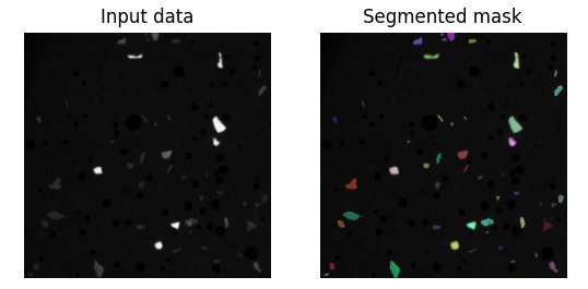
Visualization of result segmentation mask

If you want to visualize the resulting segmentation mask, you can add a small helper method to your Runner class. For example:

def visualize(self, input_data, mask):

    # Visualize the middle slice of the input data and the segmented mask
    mask_slice = mask[:, :, mask.shape[2] // 2]
    input_data_slice = input_data[:, :, input_data.shape[2] // 2]

    # Create random colors for each unique particle ID
    rng = np.random.default_rng(seed=42)
    rgb = np.zeros((*mask_slice.shape, 3), dtype=np.float32)
    ids = np.unique(mask_slice)
    ids = ids[ids != 0]
    colors = rng.random((len(ids), 3))
    for i, c in zip(ids, colors):
        rgb[mask_slice == i] = c

    # Plot input data and segmented mask
    plt.subplot(1, 2, 1)
    plt.imshow(input_data_slice, cmap='gray')
    plt.title("Input data")
    plt.axis('off')

    plt.subplot(1, 2, 2)
    plt.imshow(input_data_slice, cmap='gray')
    plt.imshow(rgb, alpha=(mask_slice > 0) * 0.5)
    plt.title("Segmented mask")
    plt.axis('off')
    plt.show()

To show this result only when debugging, we recommend using an environment variable. You can set it in the __main__ block:

import os

if __name__ == "__main__":
    os.environ["COMPOX_DEBUG_SHOW"] = "1"
    debug(
        algo_dir="algorithms/particle_seg_3d/",
        data="path to data",
        params={"particle_size": 1.0, "spacing": 0.01},
        device="gpu",
    )

Then, in your inference method, call the visualize function only when this environment variable is set:

if os.getenv("COMPOX_DEBUG_SHOW") == "1":
    self.visualize(input_data, mask_np)

This way, the visualization will appear when you run Runner.py directly for debugging, but it will not show any extra windows when the algorithm is executed from TESCAN Picannto. After running, you should see the input data on the left and segmented mask on the right:

Visualization

6. Updating the progress bar in TESCAN Picannto during inference

This step is optional. By default, the TESCAN Picannto already displays a progress bar that is updated during most stages of the algorithm execution. However, during the inference step the progress bar is not updated and only continues once inference is fully completed.

Simple progress updates inside `inference`

You can update the progress bar from anywhere inside the inference method using the set_progress function. The function accepts a floating-point value in the range 0.0 – 1.0, representing the overall progress.

# Prepare data and setup model
zarr_path, output_path = self.prepare_data(input_data, args)
self.set_progress(0.1)

# Run prediction
predict_cases(...)
self.set_progress(0.8)

# Load output as numpy array
mask_zarr = output_path / "data" / "data.zarr"
mask_np = zarr.open(mask_zarr, mode="r")[:]
self.set_progress(0.9)

The estimated remaining time is computed automatically by the TESCAN Picannto based on how often and how smoothly the progress value is updated.

More accurate progress updates using callbacks

Most of the runtime is spent inside the predict_cases function. For smoother progress updates, you can propagate a progress callback down into the prediction loop and report incremental progress during batch processing.

Create a progress callback helper in the Runner class:

def make_progress_callback(self, start, end):
    span = end - start

    def callback(frac):
        frac = max(0.0, min(1.0, float(frac)))
        self.set_progress(start + span * frac)

    return callback

Next, create a progress callback instance and pass it into predict_cases. For simplicity, we map the entire inference step to the full progress range 0.0 – 1.0:

# Run prediction
progress_callback = self.make_progress_callback(0.00, 1.00)
predict_cases(..., progress_callback=progress_callback)

To enable this, ParticleSeg3D needs a small patch to accept and forward the progress_callback. In external/particleseg3d/inference/inference.py, add an optional argument and forward it:

def predict_cases(..., progress_callback=None):
    ...
    predict_case(..., progress_callback=progress_callback)

def predict_case(..., progress_callback=None):
    ...
    predict(..., progress_callback=progress_callback)

ParticleSeg3D uses PyTorch Lightning for prediction. One simple way to track progress is to register a Lightning Callback that reports progress at the end of each prediction batch:

from pytorch_lightning.callbacks import Callback

class PredictProgressCallback(Callback):
    def __init__(self, total_steps, progress_cb):
        self.total_steps = max(1, int(total_steps))
        self.progress_cb = progress_cb
        self.seen = 0

    def on_predict_batch_end(self, trainer, pl_module, outputs, batch, batch_idx, dataloader_idx=0):
        self.seen += 1
        self.progress_cb(self.seen / self.total_steps)

Then, inside the predict function:

def predict(..., progress_callback = None) -> None:
    ...
    sampler, aggregator, chunked = create_sampler_and_aggregator(...)

    report_progress = None
    if progress_callback is not None:
        total_steps = len(sampler)
        report_progress = PredictProgressCallback(total_steps, progress_callback)
        trainer.callbacks.append(report_progress)

    try:
        model.prediction_setup(aggregator, chunked, zscore)
        trainer.predict(model, dataloaders=sampler)
    finally:
        if report_progress is not None:
            trainer.callbacks.remove(report_progress)

    #model.prediction_setup(aggregator, chunked, zscore)
    #trainer.predict(model, dataloaders=sampler)
    border_core_resized_pred = aggregator.get_output()
    ...

Note that the original trainer.predict(...) call without progress reporting should be removed or commented out to avoid running the prediction twice. This approach provides smooth and meaningful progress updates during inference, even for large volumetric datasets.

7. Algorithm Deployment

Once your algorithm is implemented and ready, you can deploy it to Compox using two options:

Single command
GUI

Option 1: Deploy with single command

Simply run this command:

compox deploy-algorithms --config app_server.yaml --name particle_seg_3d

If you are running the server for the first time, the process might take a bit longer because Compox needs to download and initialize the MinIO service.

Option 2: Deploy with GUI

As an alternative, you can use the built-in Compox GUI to manage algorithms more conveniently. First, edit your app_server.yaml file and enable GUI controls by setting the following values in the gui section:

gui:
  algorithm_add_remove_in_menus: true
  use_systray: true

Then start the Compox server with:

compox run --config app_server.yaml

After running this command, you should see the Compox icon appear in the system tray:

SysTray

Right-click the icon to open the context menu. From there, you can:

View all currently deployed algorithms
Add a new algorithm by selecting its folder (in our case, choose algorithms/particle_seg_3d)

Stopping the Server

If you are using the GUI, right-click the tray icon and select Quit to stop the server. Using Ctrl + C in the terminal will not close the server properly when the GUI mode is active.
If you are running from the terminal (without GUI), you can simply press Ctrl + C.

8. Running ParticleSeg3D in `TESCAN Picannto`

After deploying the algorithm to Compox, you can run it directly on data loaded in TESCAN Picannto.

Step 1: Start the Compox server

Before launching TESCAN Picannto, make sure the Compox is running. Start the server with:

compox run --config app_server.yaml

Step 2: Connect `TESCAN Picannto` to Compox

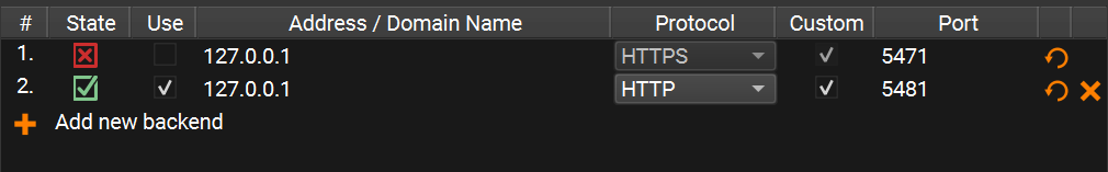
After starting the server, open TESCAN Picannto. If you see an error saying that the Compox backend connection failed, don’t worry — you can fix this by adding a new backend manually:

Go to Menu → Tools → Preferences
Click Add new backend
Set the Protocol type to HTTP
Check the Custom checkbox
Set the Port number based on your app_server.yaml file
- The default port is 5481
- If you changed it, you can verify the value in the first line of app_server.yaml

Your Preferences window should now look like this:

Preferences

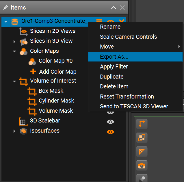
Step 3: Run the algorithm from the Compox extension

Once the backend is connected, import your dataset in TESCAN 3D Picannto.

Then open the Compox Backend Extension by clicking the Compox icon in the upper-right corner of the interface.

Preferences

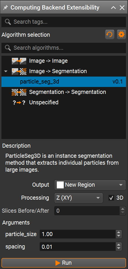
In the Compox Backend Extension window you can:

Select the algorithm you want to run
Read its description
Adjust parameters defined in your pyproject.toml file

After setting the parameters, click Run to start the inference. A progress bar should appear, and the algorithm will run on your dataset. When running ParticleSeg3D on large volumetric datasets, the choice of the particle_size parameter has a significant impact on the overall runtime. As noted by the original authors, decreasing the particle_size leads to a rapid increase in computational cost. In practice, the runtime grows almost exponentially as the target particle size becomes smaller. This effect is caused by a much higher number of patches and inference steps required to process the volume at finer spatial resolution.

Tutorials

FlowDenoising Deployment

1. Compox Installation

2. Importing FlowDenoising as submodule

3. Creating the pyproject.toml file

[project] section – basic package information

[tool.compox] section – Algorithm-specific configuration

Explanation of key fields:

4. Creating Runner.py

Importing dependencies

Initializing the Runner class

Implementing FlowDenoising in the inference method

5. Debugging Runner.py

Debug function inputs

Running debug tool

Option 1: Use the debug() Function

Option 2: Debug through the CLI

Visualization of filtered data

6. Updating the progress bar in Viewer during inference

Simple progress updates inside inference

More accurate progress updates using callbacks

Creating a progress callback helper

Passing the callback into OF_filter

Propagating progress through the filtering implementation

Reporting progress per axis

Calling progress reporting inside axis filters

7. Algorithm Deployment

Option 1: Deploy with single command

Option 2: Deploy with GUI

Stopping the Server

8. Running FlowDenoising in TESCAN 3D Viewer

Step 1: Start the Compox server

Step 2: Connect Tescan 3D Viewer to Compox

Step 3: Run the algorithm from the Compox extension

ParticleSeg3D Deployment

1. Compox Installation

2. Importing ParticleSeg3D as submodule

3. Creating the pyproject.toml file

[project] section – basic package information

[tool.compox] section – Algorithm-specific configuration

Explanation of key fields:

4. Creating Runner.py

Importing dependencies

Initializing the Runner class

Implementing ParticleSeg3D in the inference method

5. Debugging Runner.py

Debug function inputs

Running debug tool

Option 1: Use the debug() Function

Option 2: Debug through the CLI

Visualization of result segmentation mask

6. Updating the progress bar in TESCAN Picannto during inference

Simple progress updates inside inference

More accurate progress updates using callbacks

7. Algorithm Deployment

Option 1: Deploy with single command

Option 2: Deploy with GUI

Stopping the Server

8. Running ParticleSeg3D in TESCAN Picannto

Step 1: Start the Compox server

Step 2: Connect TESCAN Picannto to Compox

Step 3: Run the algorithm from the Compox extension

3. Creating the `pyproject.toml` file

4. Creating `Runner.py`

Initializing the `Runner` class

Implementing FlowDenoising in the `inference` method

5. Debugging `Runner.py`

Option 1: Use the `debug()` Function

Simple progress updates inside `inference`

Passing the callback into `OF_filter`

8. Running FlowDenoising in `TESCAN 3D Viewer`

Step 2: Connect `Tescan 3D Viewer` to Compox

3. Creating the `pyproject.toml` file

4. Creating `Runner.py`

Initializing the `Runner` class

Implementing ParticleSeg3D in the `inference` method

5. Debugging `Runner.py`

Option 1: Use the `debug()` Function

Simple progress updates inside `inference`

8. Running ParticleSeg3D in `TESCAN Picannto`

Step 2: Connect `TESCAN Picannto` to Compox